Skip to content
Flownex SE 2026 Release 2

Flownex 2026 R2 introduces major enhancements for the system-level simulation of data centre thermal-fluid systems. This release adds a dedicated suite of data centre components for modelling air-cooled and liquid-cooled racks with all the connected cooling equipment. These new components provide an optimised modelling workflow, cutting the time to setup transient digital twins by more than 50%, while still providing the same level of accuracy. Allowing engineers to rapidly evaluate the performance of different designs in complex operational conditions.

Engineers can model heat transfer, hydraulic distribution, thermal inertia and control behaviour, using manufacturer performance data with selectable modelling fidelity for detailed steady-state and transient analysis of complex cooling networks. This makes it easy to track critical results such as maximum TCS and air temperatures to evaluate designs and find issues before construction begins.

Flownex 2026 release 2

Flownex 2026 R2 introduces major enhancements for the system-level simulation of data centre thermal-fluid systems. This release adds a dedicated suite of data centre components for modelling air-cooled and liquid-cooled racks with all the connected cooling equipment. These new components provide an optimised modelling workflow, cutting the time to setup transient digital twins by more than 50%, while still providing the same level of accuracy. Allowing engineers to rapidly evaluate the performance of different designs in complex operational conditions.

Engineers can model heat transfer, hydraulic distribution, thermal inertia and control behaviour, using manufacturer performance data with selectable modelling fidelity for detailed steady-state and transient analysis of complex cooling networks. This makes it easy to track critical results such as maximum TCS and air temperatures to evaluate designs and find issues before construction begins.
major enhancements

The complete Release Notes containing detailed descriptions of the enhancements in the Flownex SE 2026 R2 version 9.1.4 are available under the Help ribbon in the latest Flownex SE release.

DC Cooling Equipment Components

A new Data Centre Cooling Equipment category has been added, with components focussed on data centre applications, as shown in Figure 1.

Figure 1: Data Centre Cooling Equipment category

The components available in the Data Centre Cooling Equipment category will be described in more detail below. The Flownex modules required for the Data Centre Cooling Equipment components are the Thermal Fluid module, Advanced Thermal Fluid module and the Control module.

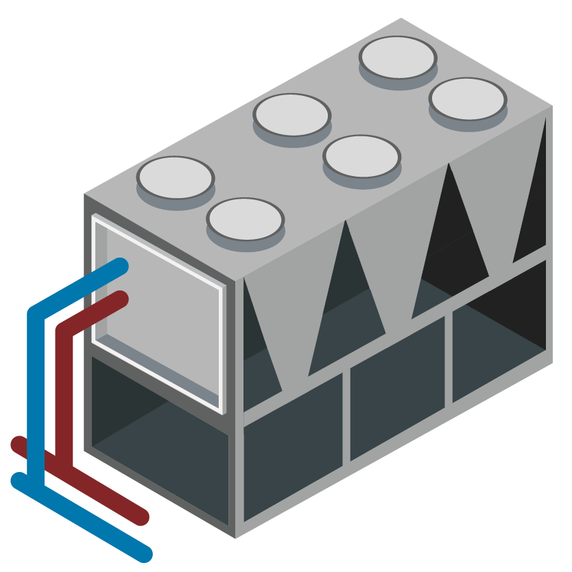
Air Cooled Chiller

The Air Cooled Chiller (ACC) component uses readily available manufacturer performance data entered in a chart to describe chiller behaviour. The component can account for varying capacity with ambient and return water conditions as well as capture the transient performance during chiller startup and restart.

Figure 2: Air Cooled Chiller
Air Cooled Data Module

The Air Cooled Data Module component models air-side heat transfer and pressure drop in a data hall using a flow network approach. The model combines the air volumes and heat from IT equipment and includes bypass and recirculation paths for cases where supply airflow is reduced or lost. This model is ideal for lower-detail use cases where CFD data is not available or when faster solving times are required.

Data Hall
Figure 3: Air Cooled Data Module
Computer Room Air Handler

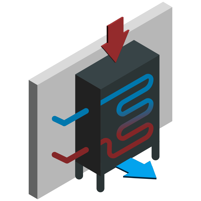
The Computer Room Air Handler (CRAH) component is a liquid-to-air heat exchanger that removes heat from data hall air and transfers it to a chilled water loop, combined with a fan component downstream of the coil that moves the air through the coil. The component contains PID control for the supply and return air temperatures using the PICV opening and fan speed. The heat exchanger can be defined using selection data and geometry, or with a single selection point if geometry data is not available.

Figure 4: Computer Room Air Handler
Coolant Distribution Unit

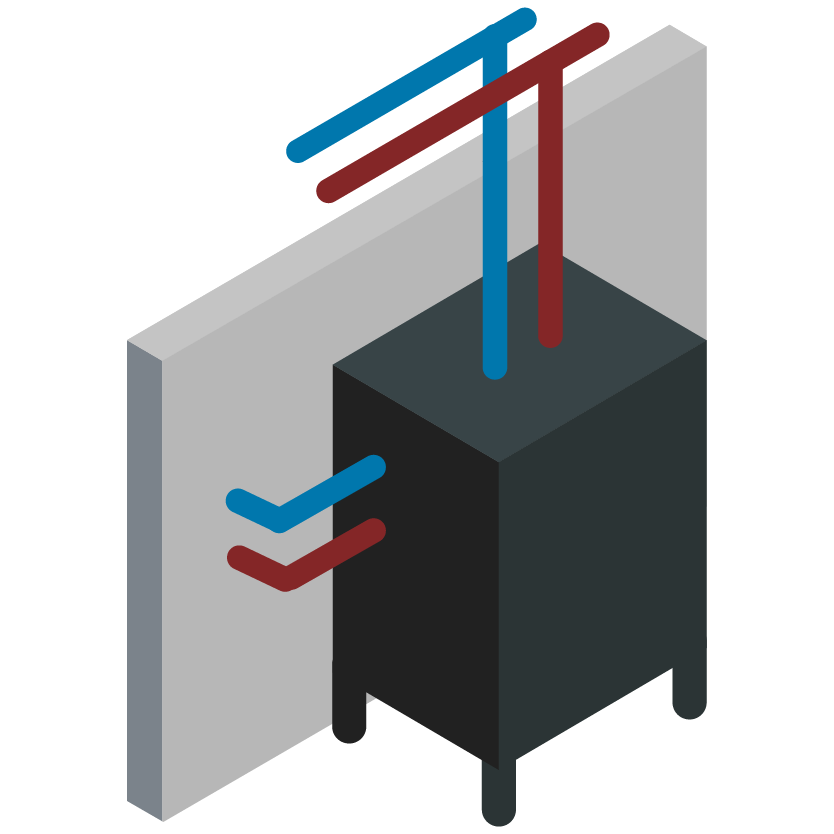
A Coolant Distribution Unit (CDU) component has been added for modelling the flow and heat transfer between TCS and FWS in liquid-cooled data centres. It combines a liquid-to-liquid heat exchanger, a PIC valve, and a TCS pump. PID control is included to vary the PIC valve opening to provide a specific TCS supply temperature. The heat exchanger is defined using readily available manufacturer data. A user can optionally include geometry so that thermal mass is included in the calculations.

Figure 5: Coolant Distribution Unit
Dry Air Cooler

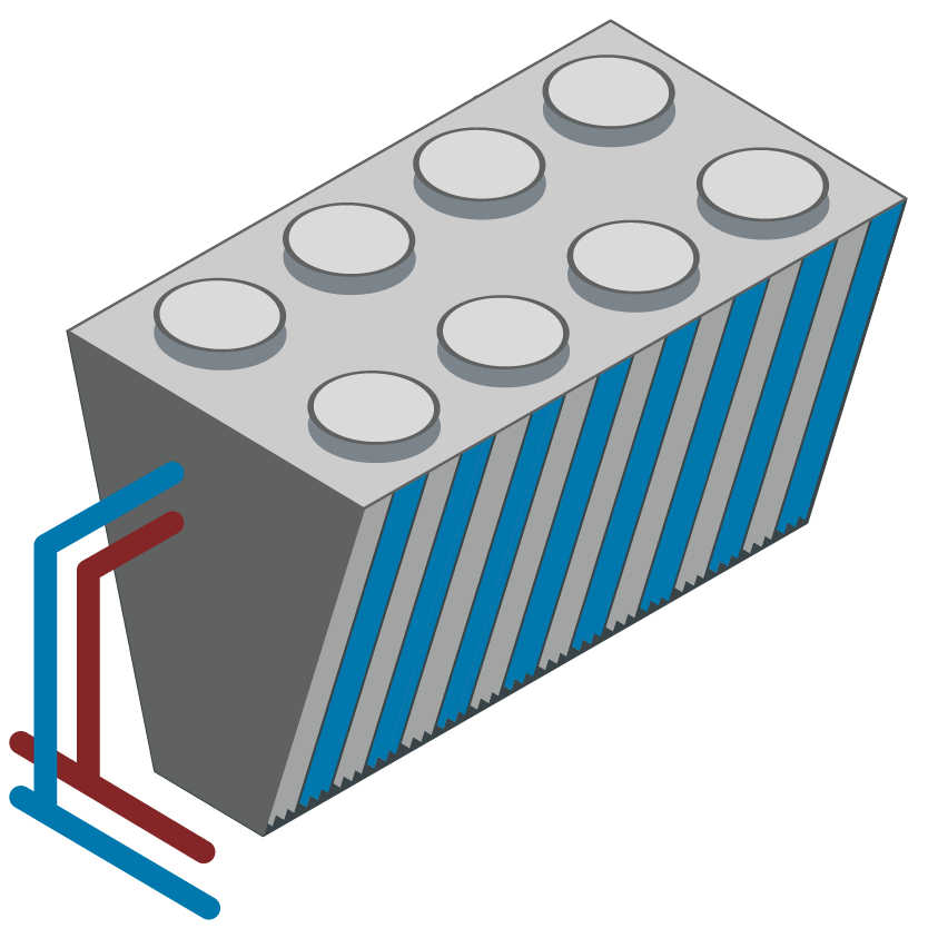
Dry Air Cooler (DAC) component models heat rejection where ambient air cools hot water circulating through a coil. The component uses a single specified operating point and calculates heat transfer and effectiveness at other operating points using the method described in VanGilder et al., 2025. 

Figure 6: Dry Air Cooler
Fan Wall Unit

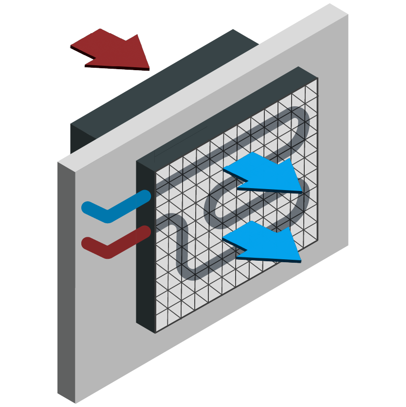
The Fan Wall Unit (FWU) component is a liquid-to-air heat exchanger that removes heat from data hall air and transfers it to a chilled water loop, combined with a fan component upstream of the coil that moves the air through the coil. The component contains PID control for the supply and return air temperatures using the PIC valve opening and fan speed. The heat exchanger can be defined using selection data and geometry, or with a single selection point if geometry data is not available.

Figure 7: Fan Wall Unit
Hybrid Dry Air Cooler

The Hybrid Dry Air Cooler (HDAC) component works like the Dry Air Cooler, with the added ability to cool the inlet air using evaporative cooling. A single specified operating point is used to calculate the off-design performance.

Figure 8: Hybrid Dry Air Cooler
Liquid Cooled IT Rack

The Liquid Cooled IT Rack component models coolant flow and heat transfer for IT equipment typically used in liquid-cooled data centres. The model accounts for the pressure drop and heat transfer in the rack using a simplified approach to capture the system-level performance. As a result, the detailed specifications of the servers are not required as inputs.
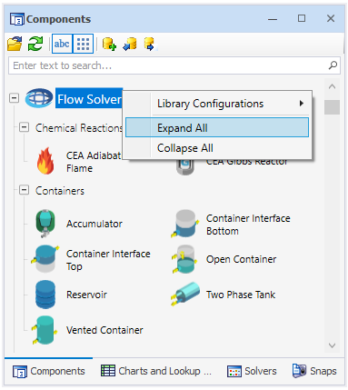
Figure 9: Liquid Cooled IT Rack
Pump with Flow Control

The Pump with Flow Control component combines a pump with PID control and adjusts pump speed to maintain a target flow rate as system conditions change. Built-in operating modes support automatic and manual control, as well as trip scenarios.

Figure 10: Pump with Flow Control
Thermal Energy Storage Tank

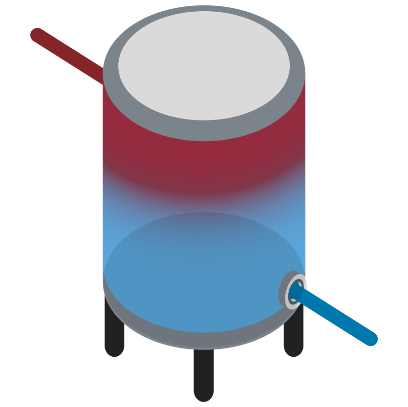
The Thermal Energy Storage (TES) Tank component models thermal stratification in a tank that can act as a buffer to protect downstream systems. The model allows different levels of stratification that range from a homogeneously mixed tank up to a perfectly stratified tank.

Figure 11: Thermal Energy Storage Tank
Water Cooled Chiller

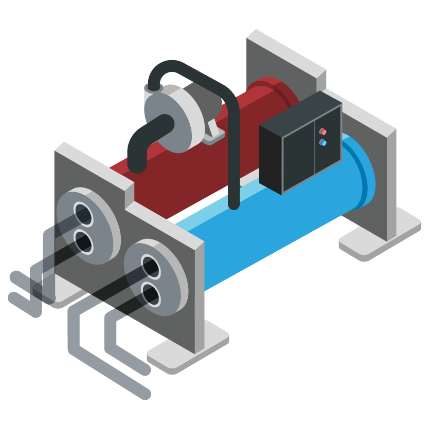
The Water-Cooled Chiller (WCC) component uses readily available manufacturer performance data entered in a chart to describe chiller behaviour. The component can account for varying capacity with condenser and evaporator temperatures as well as capture the transient performance during chiller startup and restart.

Figure 12: Water Cooled Chiller
Sub-Components

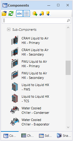
The following components were added to the “Sub-Components” subcategory as shown in Figure 13. These components are used internally in the components in the Data Centre Cooling Equipment category combined with other flow and control components, but can also be used individually.

Figure 13: Sub-Components in Data Centre Cooling Equipment Category
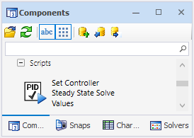
Set Controller Steady State Solve Values Script

A script component was added to the Data Centre Cooling Equipment category under a Scripts sub-category, as shown in Figure 14.

Figure 14: Set Controller Steady State Solve Values Script

Before running a transient scenario, first run a null transient (with no actions) so the PIDs can reach their setpoints. After that, the “Set Controller Steady State Solve Values” script can be run to update the “Steady state solve value” inputs on the data centre cooling components. This condition can then be saved as a snap so that future transient runs can start from this settled condition.

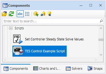
TES Control Script

An example Thermal Energy Storage Control Script (TES Control Example Script) has been added to the Data Centre Cooling Equipment category in the Scripts sub-category, as shown in Figure 15.

Figure 15: TES Control Example Script

The TES Control Example Script component provides inputs to regulate TES Tank control valve operation to achieve desired chilled water flow paths through and around TES Tanks in response to changing system conditions. The TES Control Examples Script allows the user to specify different TES Tank operating modes with associated control valve positions and to transition between the modes based on the control logic programmed in the script. 

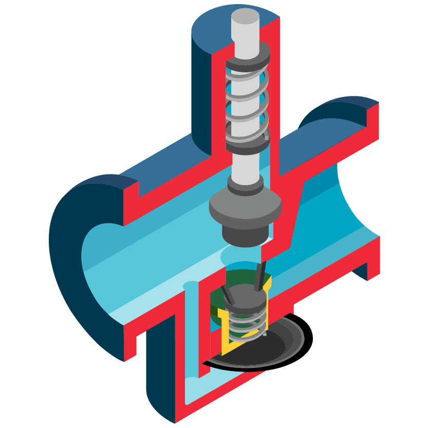
Pressure Independent Control Valve

A Pressure Independent Control Valve (PICV) was added under the Valves category. The PICV maintains a constant volume flow at a specific opening setting, regardless of the pressure difference across the valve. If the pressure difference falls below the minimum required pressure, the flow begins to decrease following typical valve flow behaviour.

Pressure Independent Control Valve (PICV)
Figure 16: Pressure Independent Control Valve added to Valves category

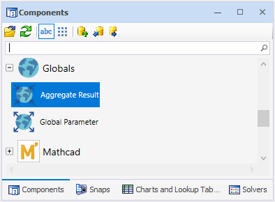
Aggregate Results

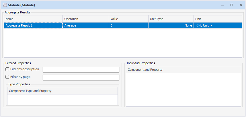
 A new Aggregate Result component has been added which can be used to easily calculate common results in a network. The Aggregate Result component is available in the Globals Component library, as shown in Figure 16.

Figure 17: Aggregate Result components in Globals library


New aggregate results can be created by either placing the Aggregate Result component on any Drawing Page or adding new items to the Aggregate Results Setup dialog, shown in Figure 19. The Aggregate Results Setup dialog is found on the Configuration ribbon, as shown in Figure 18.

Figure 18: Aggregate Results Setup
Figure 19: Aggregate Results Setup dialog


If a new Aggregate Result is added within the configuration dialog, a Drawing Page will be created named “Aggregate Results” and a new Aggregate Result component will be placed on the page, as shown in Figure 20.

Figure 20: Aggregate Result component on Aggregate Results page


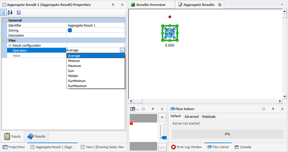
The operation to perform on the selected properties to calculate the result can be selected either on the Aggregate Result component or in the Aggregate Results Setup dialog.

The operations available are “Average”, “Minimum”, “Maximum”, “Sum”, “Median”, “RunMinimum” and “RunMaximum”. The configuration dialog can also be opened by double clicking on any Aggregate Result component.

In the Aggregate Result Setup dialog, the properties that should be used as part of the calculation can either be specified as “Individual Properties” or “Type Properties”. This allows the selection of either specific Pipe components for example, or all Pipe components.

The components that should be used can be filtered by description or by the page they are located on. The filter also supports wildcards.

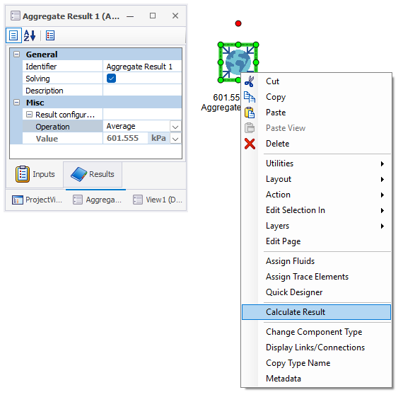
Aggregate Results will be calculated after steady state and each time step during a transient simulation, but can also be calculated at any state using the context menu, as shown in Figure 21.

Figure 21: Calculating Aggregate Results using the context menu


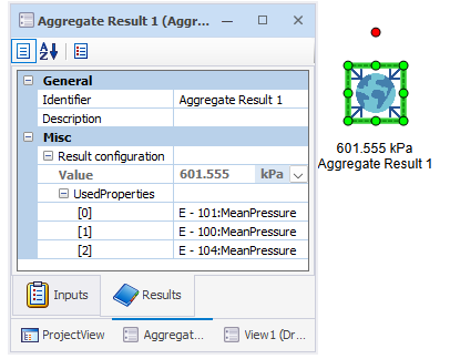
A list of the properties used in the calculation of the result is available under the Results tab for the Aggregate Result component, as shown in Figure 22.

Figure 22: Calculating Aggregate Results using the context menu

Updated Secondary Loss Factors Dialog

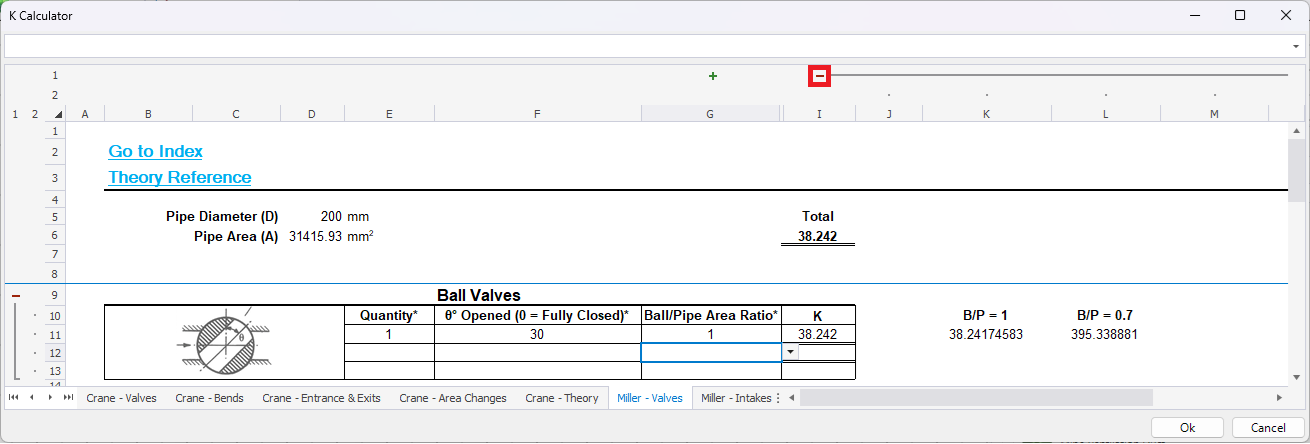
The K factor dialog for the calculation of secondary loss factors has been updated with the latest publications from:

  • Flow of Fluids through valves, pipes, pumps and fittings, TP410 2022 by CRANE Co.
  • Internal Flow Systems. D.S. Miller, 4th

An Index sheet has also been added that provides a summary of the secondary loss factors and links have been added for faster navigation.

Figure 23: Secondary Loss Factor Index

The calculation formulas can now be inspected and verified by expanding the Formula and Error Checking sections, as shown in Figure 24.

Figure 24: Formula section expanded

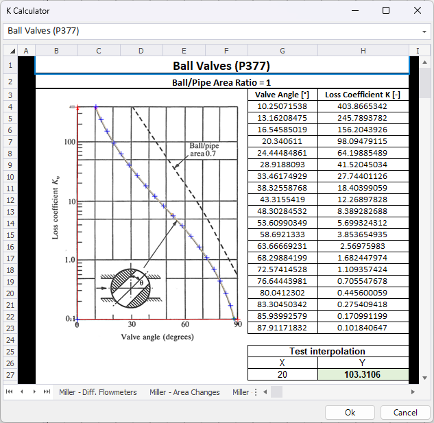
The digitisation of the source data is also now available for inspection, as shown in Figure 25, by selecting the “Information” link on a sheet.

Figure 25: Digitised source data
minor enhancements

Global Parameters

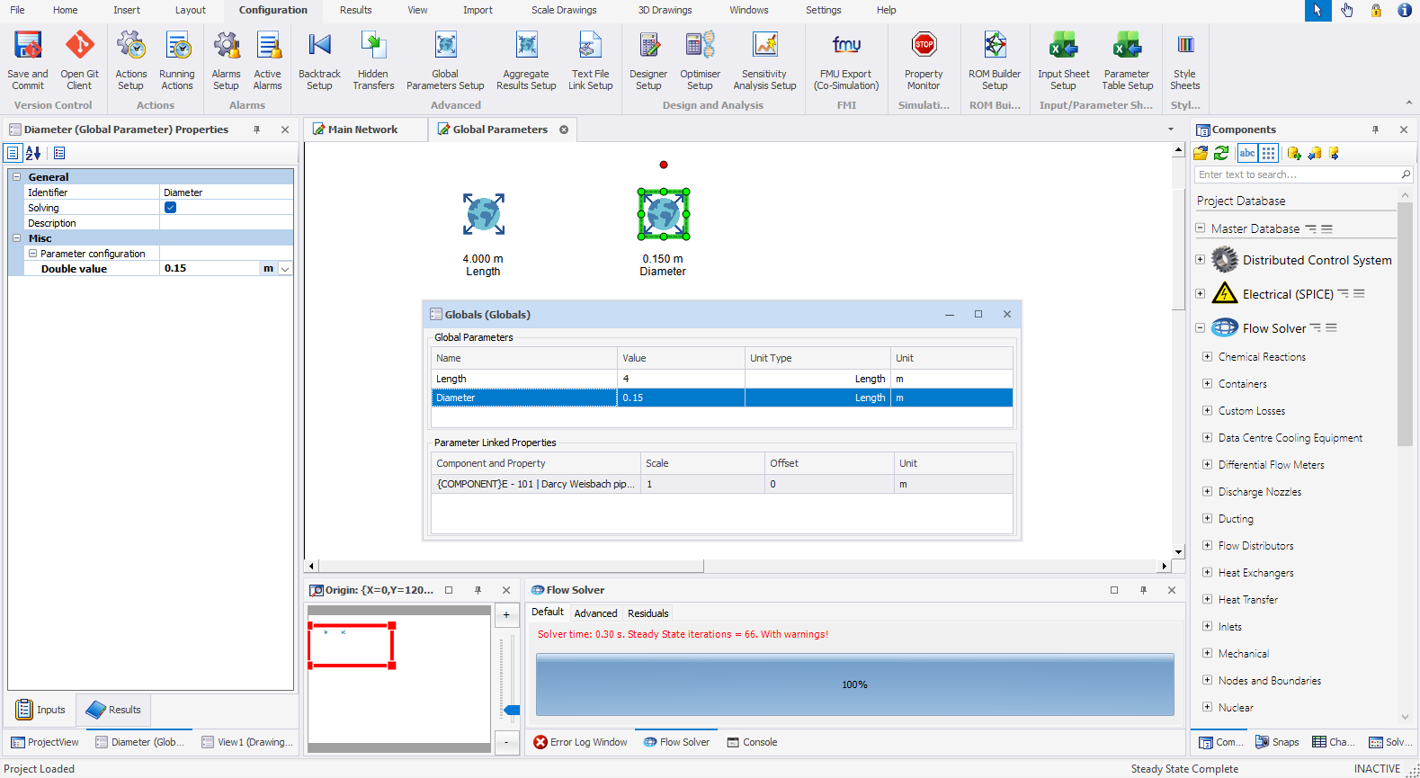
When a new Global Parameter is created in the Global Parameters Setup dialog, the Global Parameter will now be represented as a new component.

The Global Parameter component will be added to a Drawing Page named “Global Parameters” that will automatically be created in the project, as shown in Figure 26. Each Global Parameter will create a new Global Parameter component on the page.

Figure 26: Global Parameters represented as components


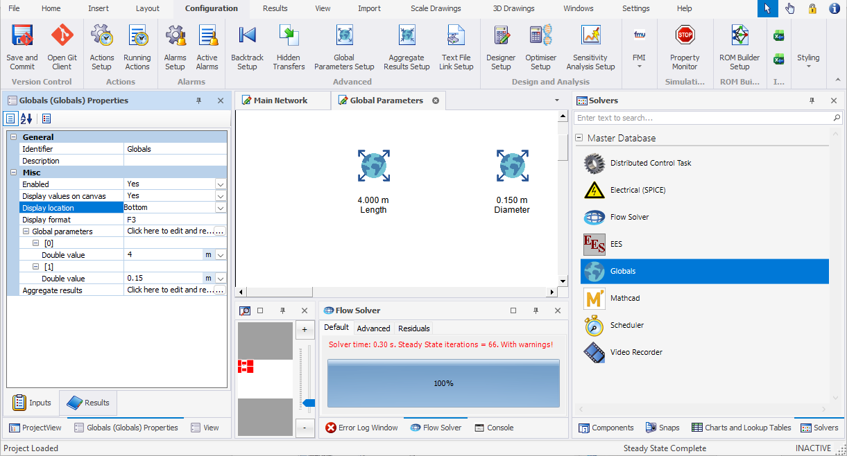
Global Parameter components will display their current value on the Global Parameters page. The display options can be edited on the Globals Properties settings, as shown in Figure 27.

Figure 27: Globals Properties settings


As Global Parameters are now components, the Value property on the Inputs page of a Global Parameter can be used like any other property in Flownex, in Actions, Designers, Sensitivity Analysis, Parameter Tables, etc.

A Global Parameter component is also available in the Components Library, and the component can be dragged and dropped on to a Drawing Page, as shown in Figure 28.

Figure 28: Global Parameters component in Components Library


Double clicking on any Global Parameter component will open the Global Parameter editor that was used in previous versions and select the corresponding Global Parameter.

Global parameters can now be used for double, integer, boolean, option, string and data reference values.

Bulk Renaming Update

The bulk renaming utility is now accessible directly from the Settings ribbon within the General group, as shown in Figure 29.

Figure 29: ID Bulk Rename in Settings ribbon


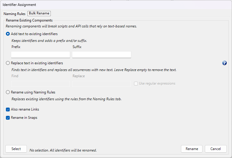
A “Select” button has been added to the Identifier Assignment dialog that allows a user to apply filters using the Find dialog to rename a targeted subset of project components and links. Renaming operations can be restricted by page, component type or other criteria.

Figure 30: Identifier Assignment dialog

Renaming Components in Snaps

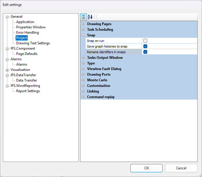
An option “Rename identifiers in snaps” has been added to automatically propagate renaming of components to snaps. A component that is renamed will be renamed in all existing snaps too when this option is enabled. The option is disabled by default and can be found under the Project Settings, as shown in Figure 31.

Figure 31: Rename identifiers in snaps setting in Project Settings

Create View Page

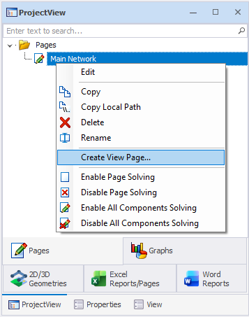
A page with View components can now be created for components on a Drawing Page or 2D/3D Geometries pages. The page can be created by selecting the “Create View Page” option that has been added to the context menu of a Drawing Page, shown in Figure 32.

Figure 32: Create View Page option on context menu

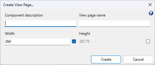
View components will then be created for components that have a description that is similar to the “Component description” specified in the Create View Page dialog, shown in Figure 33, to filter the components for which Views should be created.

Figure 33: Create View Page dialog

Drawing Utilities

Utilities have been added to the context menu when right-clicking on a Drawing Page, as shown in Figure 34.

Figure 34: Utilities option in context menu

The available utility options will be described in more detail below.

Connect Links to Nearby Nodes

This utility will link all the disconnected links to the nearest Node available.

Delete Disconnected Components

This utility will remove all components whose links are not connected to other components, along with their associated default links.

Align Links With Flow

This utility can be used to change the link directions to be in the same direction as the flow direction for a component.

Graph Digitiser Enhancements

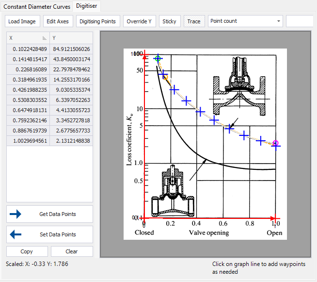
The Graph Digitiser has been enhanced with automatic line tracing, improved point editing and selection, and more efficient digitisation.

  • Line tracing: Automatically traces the centre of a graph line and generates points according to configurable criteria, including point count, point distance and maximum deviation. Existing points can also be aligned to the traced line.
Figure 35: Line tracing option in Digitiser
  • Point editing and selection: Use the arrow keys to adjust individual or multiple selected points with pixel-level precision. Hold Ctrl to select multiple points for moving or deletion. Press Esc to clear the selection, or select an individual point without holding Ctrl. Use Tab to move to the next selected marker. The context menu also includes Select all and Delete selected options.
  • Sticky mode: Automatically identifies the centre of a nearby graph line, allowing points to be placed without precise cursor positioning or excessive zooming.

Components Library Display Options

Buttons have been added for “Multi Column Display” and “Show Component Text”, as shown in Figure 36. By selecting the “Multi Column Display” button, components can now be viewed in columns and component names can be hidden by disabling “Show Component Text”.

Figure 36: Multi Column Display and Show Component Text buttons

Options have also been added to expand all levels, and collapse all sub-levels, as shown in Figure 37.

Figure 37: Expand All and Collapse All Context menu options

Property Grid Display

The Inputs and Results property grids were changed to tab pages, as shown in Figure 38, which provide more space for the properties in the grids.

Figure 38: Inputs and Results tab pages

Project View Display

The Project View page navigation buttons have been replaced with tabs, as shown in Figure 39. This allows for more space for key information on smaller screens.

Figure 39: Project View page navigation tabs

Graphs

Graphs can now be added from the context menu on the property grid. Multiple properties can also be selected to be added to graphs.

Figure 40: Adding graphs from the context menu on the property grid

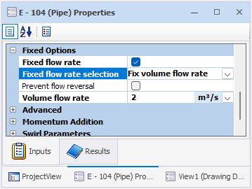
Fixed Volume Flow

Fixed volume flow can be specified on flow elements in the same way that fixed mass flow can be specified, as shown in Figure 41.

In the case of a fixed element volume flow rate, the solver compensates for varying density in the element, thereby keeping volumetric flow rate fixed whilst satisfying continuity. Typical applications for this functionality are positive displacement pumps and fans.

Figure 41: Fix volume flow rate option

Disable Page Solving

The following enhancements have been made to disabling page and components solving:

  • When “Disable Page Solving” is selected on a Drawing Page, a red cross will now be displayed over the entire Drawing Page, as shown in Figure 42.
  • The icons in the pages tree are also now distinct for the different types of disabling.
Figure 42: Disabled Drawing Page with red cross over entire Drawing Page

Project Saving to OneDrive

The compatibility has been improved when saving a Flownex project in OneDrive folders.

Quick Python Script

The Parent pointer has been made available in the Quick Python Script. This is useful when issuing warnings or errors.

Figure 43: Parent pointer available in Quick Python Script

Autodesk Revit

The following enhancements have been made:

Revit 2027 Support
  • The latest Revit version (Revit 2027) is now supported.
  • Revit moved the plugin folder from “C:\ProgramData\Autodesk\Revit\Addins” to “C:\Program Files\Autodesk\Revit 2027\AddIns” of which the latter requires administrator rights to modify. The FlownexSE Revit installer function will detect this and attempt to install the FlownexSE plugin into Revit with an elevated PowerShell prompt. If a user does not have administrative rights, the installation will fail.
COM Compatibility Test

The Revit extension will now test if the COM registered FlownexSE version is compatible with the Revit plugin. If the version is not compatible, an error message will be issued so that the user can take corrective action. The versions will also be displayed in the Flownex Network Builder window, as shown in Figure 44. The first three numbers of the version, for example “9.1.2”, must be the same for successful communication.

Figure 44: Versions displayed in the Flownex Network Builder window

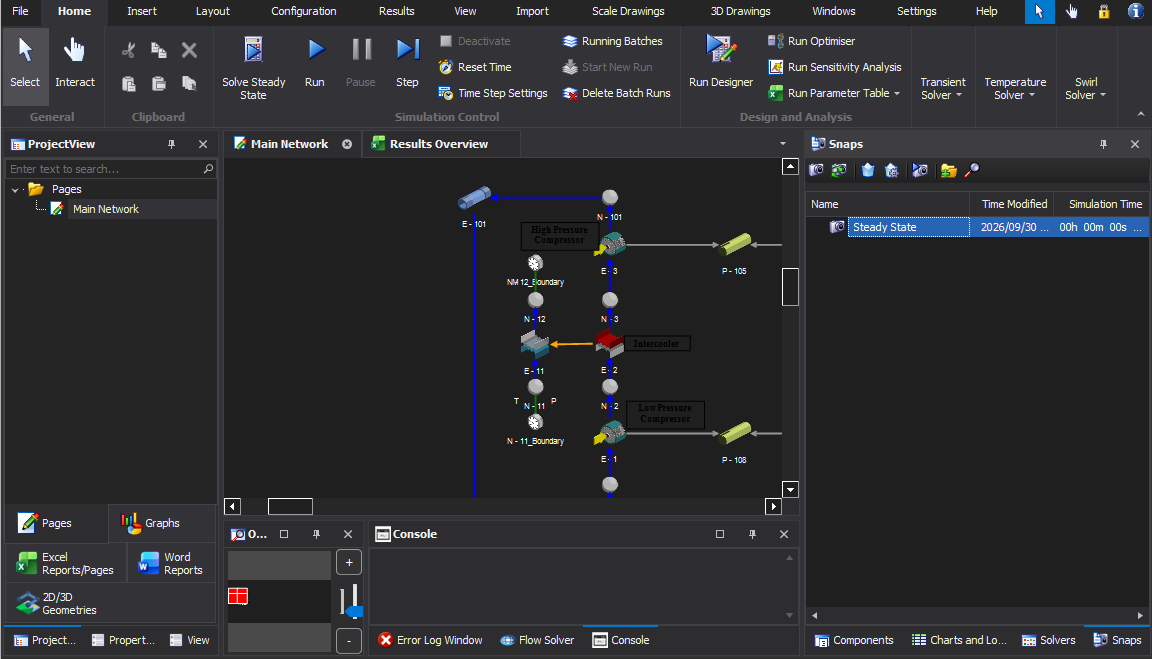
Dark Mode

The following enhancements have been made when Dark Mode is used:

  • The visibility of the active ribbon tab has been improved by making the name of the tab bold, as shown in Figure 45.
  • The appearance of snaps has also been improved in Dark Mode, as shown in Figure 45.
Figure 45: Dark Mode enhancements

3D View

The capability has been added to show disconnected components and hide components for which solving has been disabled in 3D view.

Components configured with variable diameters such as Gradual Pipe Transitions are now rendered dynamically in the 3D view to accurately reflect their physical geometry and tapered transitions.

Control System Step Factor

The capability has been added to run the Control System at a different timestep than the rest of the simulation through a Step factor, as shown in Figure 46.

Figure 46: Step factor option in Distributed Control Task

A step factor of 3 means the control system will only execute every 3rd step. If the main step size is 100ms then it will be 300ms for the control system. The Step factor is set on the Distributed Control Task Solver properties, with a default Step factor of 1.

Flow Conduit Links

The Flow Conduit links are no longer available by default. They can be enabled in the Project Settings by specifying “Allow flow conduit links” as “True”, as shown in Figure 47. Existing projects with flow conduit links are unaffected.

Figure 47: Allow flow conduit links setting in Project Settings

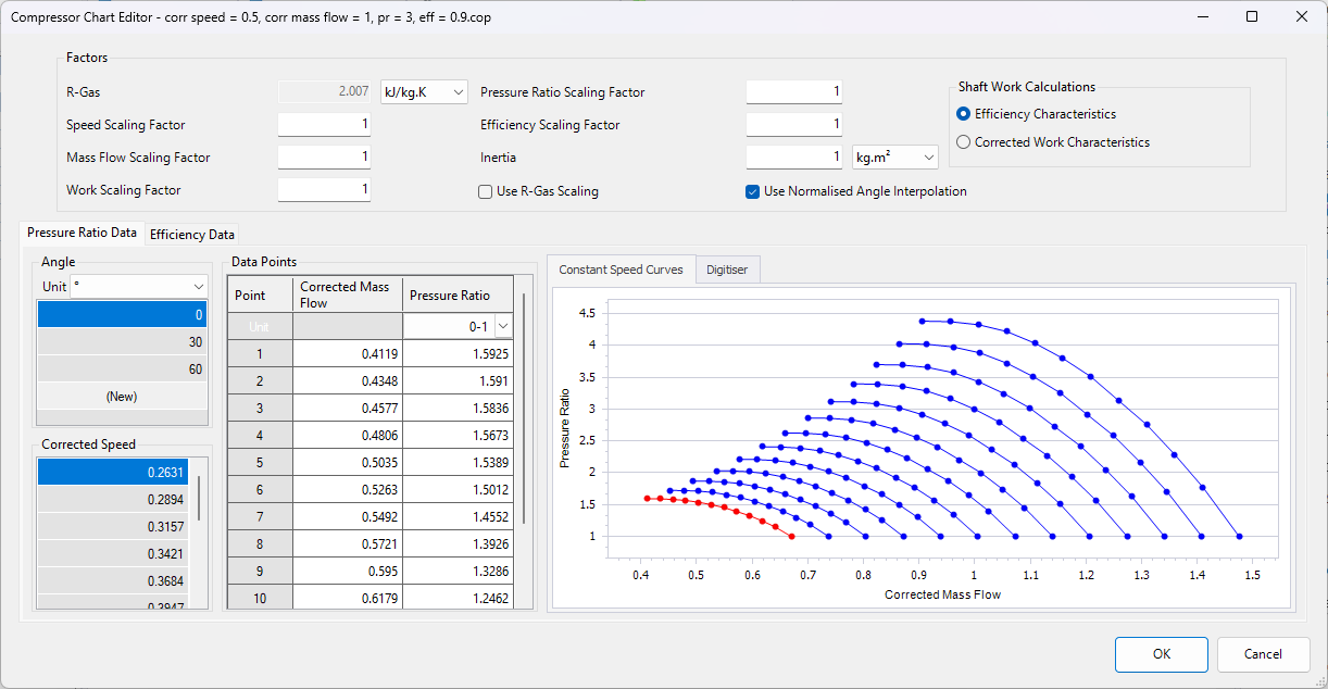
Normalised Compressor Angle Interpolation

The capability has been added to normalise interpolated curves when interpolating between neighbouring angles, similar to how it is done for interpolation between speed curves. This leads to improved boundedness and therefore accuracy in general.

Figure 48: “Use Normalised Angle Interpolation” option on Compressor Chart

Single-File Project

The working directory for .projz single-file projects can now be set to either the User Temp directory or a Custom directory (the .projz file location remains the default).

Uncoupling working files from the project archive location resolves several operational issues:

  • Cloud Syncing: Prevents OneDrive file-locking conflicts, speeds up synchronisation, and maintains clear version histories.
  • Clean Workspaces: Prevents leftover _project directories from remaining behind after executing projects with scripts.
  • Source Control: Allows the Flownex GitClient to commit changes without requiring Flownex to be closed or the _project directory to be manually deleted.
  • Data Safety: Eliminates accidental deletion of adjacent files located alongside the .projz archive.
Figure 49: “Working directory location” option in Settings

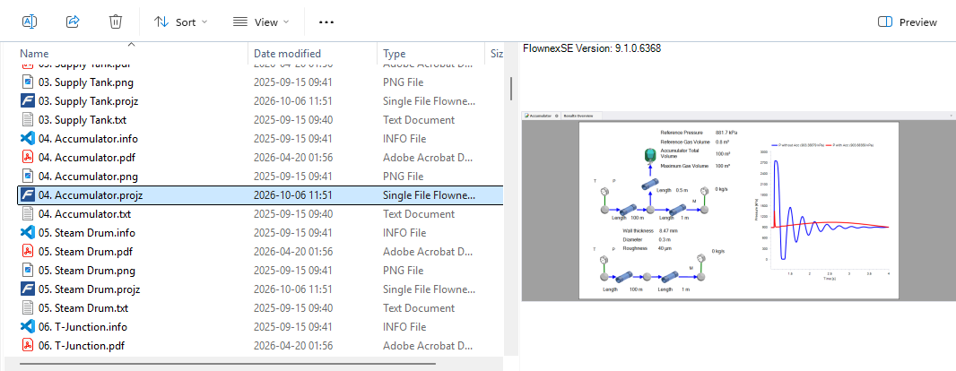
Windows File Explorer preview support has been extended to .projz single-file projects, enabling quick file previewing directly from the desktop environment, as shown in Figure 50.

Figure 50: Windows File Explorer preview support for .projz files

Remote gRPC Launcher Service

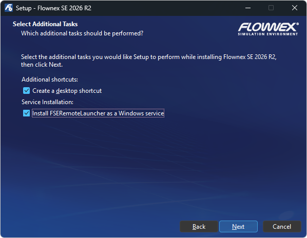
A new Windows service, FSERemoteLauncher, can be installed with Flownex SE. It lets API clients, local or over the network, start Flownex SE in the user’s session, find free ports, and wait for the gRPC API server to be ready, before connecting with the existing Flownex API.

Figure 51: Install FSERemoteLauncher option

API

Support has been added for executing custom script code through the Network Builder API. This significantly extends remote automation capabilities, enabling workflows and functionality that go beyond the scope of traditional API calls.

Find

Link Status Filter

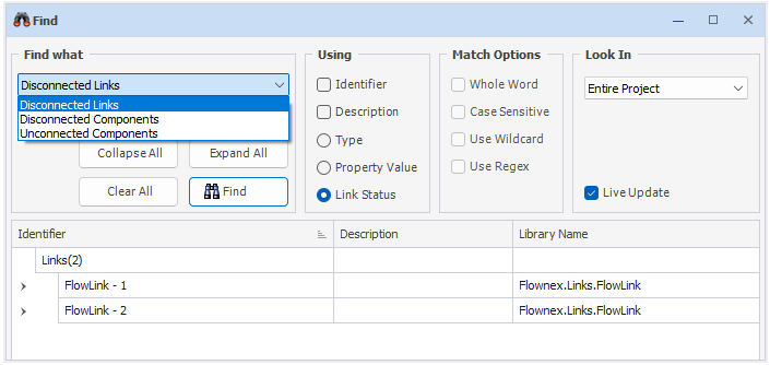
A new Link status filter has been added to the Find dialog, as shown in Figure 52, to quickly identify disconnected or incomplete network elements. The different filter options available are:

  • Disconnected Links: Links that are not connected at both ends.
  • Disconnected Components: Components with attached links that are not connected to other components.
  • Unconnected Components: Standalone components with no attached links.
Figure 52: Link Status filter in Find dialog
Live Update

A new “Live Update” option has been added to update search results after any search criteria that change to eliminate the need to repeatedly press the “Find” button. This feature can be enabled by checking the “Live Update” checkbox.

Type Search

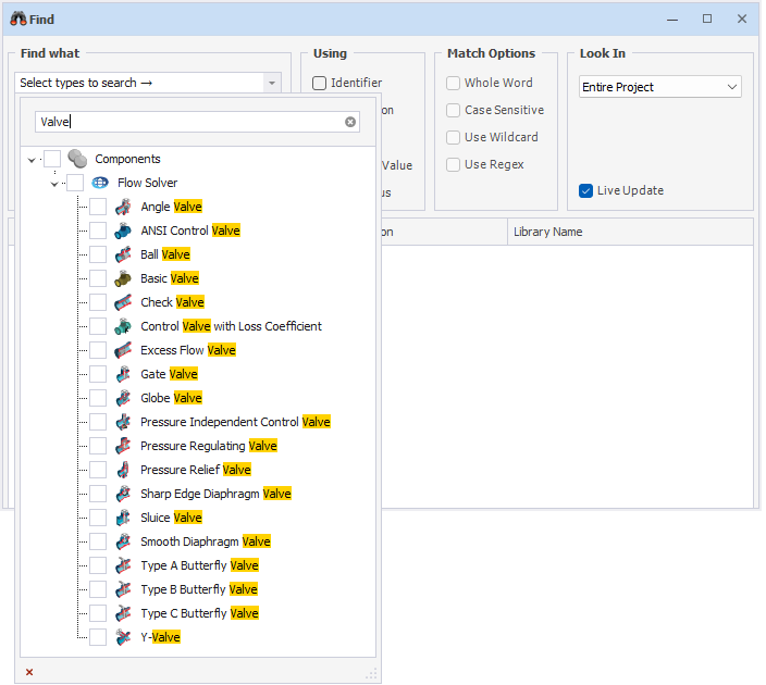
A search function has been added to the “Type” search option, as shown in Figure 53.

Figure 53: Search field available in "Type" search dropdown

CFX

Co-simulation support has been added for Ansys CFX 2026 R1.

Psychrometric Boundary Condition

The humidity ratio input can now be specified on the Psychrometric Boundary Condition above the critical temperature.

Piping

The Roughness/Diameter ratio result has been included in the Darcy Weisbach roughness warning.

WELCOME BACK

Not a user yet?  Register.

Global Flownex Websites

WELCOME BACK

Not a user yet?  Register.